Benchmarking
Table of Contents
- Evaluation
- Problems in the Water
- Using historical data as a solution
- Shrinking the benchmark as a solution
- Using dynamic benchmarks as a solution
benchmark [noun] A standard point of reference against which things can be compared. A benchmark consists of dataset(s), metric(s), and a way to aggregate performance.
Evaluation
Human evaluation is the gold standard in many NLP tasks but it suffers from prohibitive costs and poor scalability (Zouhar et al, 2026). In the absence of human supervision, researchers rely on benchmarking and automated metrics (Zouhar et al, 2026).
It comes to no surprise then dayasets are the telescopes of our field (Joshi); without reliable benchmarks, we are just like “astronomers wanting to see the stars but refusing to build telescopes” (Joshi). AI benchmarks have become the primary instrument for evaluating model capabilities, comparing AI systems, and informing deployment decisions (Jiang et al, 2026).
Problems in the Water
Inaccurate
Benchmarks often fail to measure the intended capability. Evaluation quality can degrade due to labelling errors and benchmark saturation.
Saturation Recent models have “outpaced the benchmarks [that] test them” (AI Index Report, 2021).
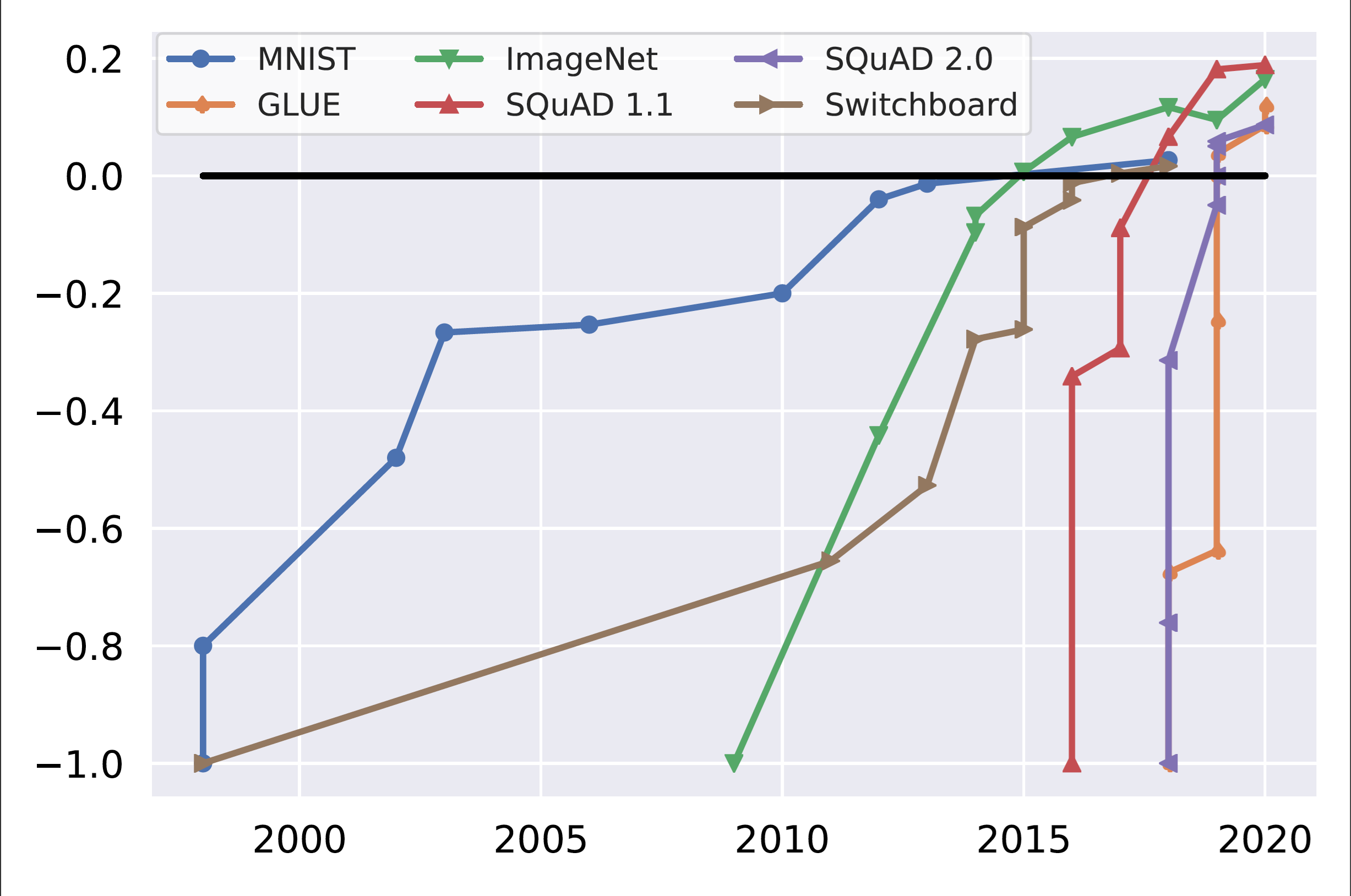 Benchmark saturation over time for popular benchmarks. Initial performance and human performance are normalized to -1 and 0, respectively (Kiela et al, 2021)
Labelling Errors
Reward Hacking
Exepnsive
Energy Evaluating generative AI models is a routine but resource-intensive, process that is conducted over and over again during the course of model development (Fisch et al, 2026).
Data Benchmarks require so much so much data that it sidelines low-resource languages. Multilingual models are evaluated only on a small subset of languages. There is no guarantee that performance on English-Spanish, the only common evaluation dataset, is representative of the expected performance of the models over all other language pairs (Anastasopoulos and Neubig, 2020).
Citations
AI Index Report (2021). ?
Anastasopoulos and Neubig (2020). ?
Fisch et al (2026). CollabEval: Statistically Efficient Collaborative Model Evaluation via Matrix Completion
Jiang et al (2026). ?
Jiela et al (2021). ?
Kiela et al (2021). ?
Zouhar et al (2026). How to Select Datapoints for Efficient Human Evaluation of NLG Models?
Using historical data
The Page 18
Citations
Fisch et al (2026). CollabEval: Statistically Efficient Collaborative Model Evaluation via Matrix Completion
Dynamic Benchmarks
Item Response Theory
Table of Contents
Item Response Theory explains the relationship between an individual’s ability and their observed performance (Columbia University Mailman School of Public Health, n.d.). Formally, the probability of correctly answering an item is a function of the person’s ability and visualized as the item response curve.
A person’s “ability” and an item’s parameters are organized on an unobservable continuum (Columbia University Mailman School of Public Health, n.d.). The main purpose of IRT is to establish an individual’s position on that continuum (Columbia University Mailman School of Public Health, n.d.).
Glossary
| Term | Definition |
|---|---|
| $i$ | subject $i$ |
| $j$ | item $j$ |
| $N$ | number of subjects |
| $M$ | number of items |
| $a_j$ | (item) discrimination parameter |
| $b_j$ | (item) difficulty parameter |
| $c_j$ | (item) guessing parameter; the chance of a correct response for a very low $\theta$ |
| $d_j$ | probability of endorsing an (item) incorrect answer in spite of high ability |
| $D=1.7$ | scaling constant |
| $\theta_i$ | (subject) ability. Formally cited as $\theta \in (-\infty, \infty)$, it more often is the case $\theta \in [-3, +3]$. An estimated ability of 1.2 can be interpreted as 1.2 standard deviations above the average ability in the population. |
| $\mathbf{r}_{ij}$ | response from subject $i$ to item $j$ |
Assumptions
- Monotonicity: As the trait level “increases,” the probability of a correct response increases.
- Unidimensionality: There is one dominant latent trait being measured and this trait is the driving force for the responses observed for each item in the measure.
- Local independence: Responses given to separate items in a test are mutually independent given a certain level of ability.
- Invariance: We can estimate item parameters from any position on the item response curve. Put another way, invariance means that item parameters do not depend on the characteristics of a particular population. Parameter invariance is crucial if one wants to carefully assess the degree of inferential generalizability across examinee populations; if parameters are not invariant, the statistical foundation for inferences is not identical across populations and hence the inferences are not generalizable across those to the same degree (Rupp and Zumbo, 2006).
Models
Unidimensional, Dichotomous
| Parameter | Formula |
|---|---|
| 1PL | $\mathbb{P}[\mathbf{r}_{ij}=1 \mid \theta_i, b_j] = \frac{\exp(D(\theta-b_j))}{1+\exp(Da(\theta-b_j))} = \frac{1}{1+\exp[-Da(\theta_i-b_j)]}$ |
| 2PL | $\mathbb{P}[\mathbf{r}_{ij}=1 \mid \theta_i, a_j, b_j] = \frac{\exp(\theta_i-b_j)}{1+\exp[a_j(\theta_i-b_j)]} = \frac{1}{1+\exp[-Da_j(\theta_i-b_j)]}$ |
| 3PL | $\mathbb{P}[\mathbf{r}_{ij}=1 \mid \theta_i, a_j, b_j, c_j] = c_j + (1-c_j)\frac{1}{1+\exp[-Da_j(\theta_i-b_j)]}$ |
| 4PL | $\mathbb{P}[\mathbf{r}_{ij}=1 \mid \theta_i, a_j, b_j, c_j, d_j] = c_j + (d_j-c_j)\frac{1}{1+\exp[-Da_j(\theta_i-b_j)]}$ |
Optimization
Notes on Joint Maximum Likelihood, conditional maximum likelihood, and marginal maximum likelihood are pulled from Johnson (2007)
Joint Maximum Likelihood
The joint maximum likelihood (JML) estimation procedure treats both item parameters and ability as unknown but fixed model parameters.
\[\left(\hat a, \hat b, \hat c, \hat d, \hat \theta \right) = \operatorname*{argmax}_{a, b, c, d, \theta} \mathcal{L}(a, b, c, d, \theta \mid \mathbf{R}) = \operatorname*{argmax}_{a, b, c, d, \theta} \prod_{i=1}^N \prod_{j=1}^M \mathbb{P}[\mathbf{r}_{ij}=1 \mid a_j, b_j, c_j, d_j, \theta_i]^{\mathbf{r}_{ij}} \left(1-\mathbb{P}[\mathbf{r}_{ij}=1 \mid a_j, b_j, c_j, d_j, \theta_i]\right)^{1-\mathbf{r}_{ij}}\]A unique solution exists if further constraints are placed on examinee and item parameters. For two parameters like the 2PL, two constraints are necessary
- a location constraint: constrain a single difficulty to some fixed dumber or the average difficulty to some number
- a scale constraint: force the product of the discrimination parameters to one $\prod_{j=1}^M a_j=1$.
Estimates are inconsistent (Neyman and Scott 1948; Andersen 1970; Ghosh 1995 from Marginal Maximum Likelihood Estimation of Item Response Models in R by Matthew S Johnson); no matter how many individuals are included in the sample, the estimates may still be biased.
Conditional Maximum Likelihood
Andersen (1970) proposed Conditional Maximum Likelihood (CML). This method conditions on the vector of raw scores $\mathbf{R}_{i+} = \sum_j \mathbf{r}_{ij}$ which is a sufficient statistic and substitute for the abilities of individuals in the sample.
Andersen (1970) shows that maximizing the objective below results in consistent item difficulties.
\[\hat b = \operatorname*{argmax}_{b} \mathcal{L}(b \mid \mathbf{R}) = \operatorname*{argmax}_{b} \prod_{i=1}^N \mathbb{P}[\mathbf{r}_i \mid b, \mathbf{R}_{i+}] = \frac{\exp\left(-\sum_j \mathbf{r}_{ij} b_j\right)}{\sum_{\{\mathbf{y}\,:\, \sum_j y_j = \mathbf{R}_{i+}\}} \exp\left(-\sum_j y_j b_j\right)}\]Note that this does not depend on the individual’s ability $\theta$. An ad hoc procedure must be implemented to estimate the ability of individuals.
In addition, the conditional maximum likelihood only works when there is a simple sufficient statistic, like the raw score for the Rasch model. More complex IRT models, including the 2 PL, do not have simple sufficient statistics.
Marginal Maximum Likelihood
Unlike joint maximum likelihood estimation techniques, the marginal maximum likelihood (MML) treats only $N$ individuals as the observational units. To accomplish this, MML assumes that abilities are sampled from some larger distributions denoted as $F(\theta)$. Typically, IRT modelers assume that the distribution F is the normal distribution with mean 0 and standard deviation 1. However the normal distribution does not necessarily work for all applications
\[(\hat a, \hat b, \hat c, \hat d) = \operatorname*{argmax}_{a,b,c,d} \mathcal{L}(a, b, c, d \mid \mathbf{R}) = \prod_i \mathbb{P}[\mathbf{r}_{i} \mid a, b, c, d] = \prod_i \int_\theta L_i(\theta_i \mid \mathbf{r}_i, a, b, c, d)dF(\theta_i)\]Like the JML estimation method, location and scale constraints are required to achieve a unique solution. The constraints can either be placed on the means and standard deviation of the ability distribution $F(\theta)$ or on the item parameters.
Variatonal Inference
Wu et al. (2020) proposed VIBO, a variational inference method for fitting IRT models to large datasets. Applying this method to five large-scale item response datasets from cognitive science and education yields higher log likelihoods and improvements in imputing missing data.
The authors made the assumptions listed below
$\theta_i \in \mathbb{R}^{K} : \mathbb{P}[\theta_i] = \prod_{k=1}^K \mathbb{P}[\theta_{i,k}]$ where $\mathbb{P}[\theta_{i,k}] \sim \mathcal{N}(0,1)$
$\mathbb{P}[\{a_j, b_j, c_j, d_j\}_{j=1:M}] = \prod_{j=1}^M \mathbb{P}[{a_j, b_j, c_j, d_j}]$ where $\mathbb{P}[{a_j, b_j, c_j, d_j}] \sim \mathcal{N}(0,1)$
$q_\phi(\{a_j,b_j,c_j,d_j\}_{j=1:M} | \mathbf{r}_{i,1:M}) = q_\phi(\{a_j,b_j,c_j,d_j \}_{j=1:M}) = \prod_{j=1}^M q_\phi(\{a_j,b_j,c_j,d_j \}_{j=1:M})$
The goal of VIBO is to pick a family of distribution that “best approximates the true posterior by minimizing an estimate of mismatch between true and approximate distributions.” Observed variable $x \in \mathcal{X}$ represents responses from a single student $\mathbf{r}_i$ and latent variables $z \in \mathbf{\mathcal{Z}}$ represents ability and item characteristics $\theta_i, \{a_j,b_j,c_j,d_j\}_{j=1:M}$.
\[q_{\psi^*(x)}(z)=\operatorname*{argmin}_{q_{\psi(x)}} D_{\text{KL}}\big(q_{\psi(x)}(z),|,p(z|x)\big)=\operatorname*{argmax}_{\psi(x)}\mathbb{E}{q_{\psi(x)}(z)}\left[\log\frac{p(x,z)}{q_{\psi(x)}(z)}\right]\]by definition: minimizing the KL-divergence to the log posterior is equivalent to maximizing the ELBO
Let $\mathbb{P}_D(x)$ be an empirical distribution over the observed variables. The average quality of the variational approximations is
\[\mathbb{E}_{\mathbb{P}_D(x)}\left[\max_{\psi(x)} \mathbb{E}_{q_{\psi(x)}(z)}\left[\frac{\mathbb{P}[x,z]}{q_{\psi(x)}(z)}\right]\right]\]Learning an approximate posterior for each $x \in D$ can grow to be unwieldy in a large dataset. Wu et al. (2020) proposed an amortized function $f_\phi$ (parameterized by $\phi$) that maps a person’s responses directly to parameters of their approximate posterior distribution. The number of parameters in amortization is vastly smaller than learning a per-observation posterior.
\[\max_\phi \mathbb{E}_{\mathbb{P}_D(x)}\left[\mathbb{E}_{q_\phi(z|x)}\left[\log \frac{\mathbb{P}[x,z]}{q_\phi(z|x)}\right]\right]\]Wu et al. (2020) proved that VIBO is a lower bound on the log marginal probability of person $i$’s response.
\[\begin{flalign} \log \mathbb{P}_\theta[\mathbf{r}_{i,1:M}] \ge \text{VIBO} &\triangleq \mathcal{L}_{\text{recon}} + \mathbb{E}_{q_\phi(\{a_j,b_j,c_j,d_j\}_{j=1:M}|\mathbf{r}_{i,1:M})}[D_{\text{ability}}] + D_{\text{item}} \\ \mathcal{L}_{\text{recon}} &= \mathbb{E}_{q_\phi(\theta_i, \{a_j, b_j, c_j, d_j\}_{j=1:M}|\mathbf{r}_{i,1:M})}\left[\log \mathbb{P}_\theta[\mathbf{r}_{i,1:M}|\theta_i, \{a_j, b_j, c_j, d_j\}_{j=1:M}]\right] \\ D_{\text{ability}} &= D_{\text{KL}}\left(q_\phi(\theta_i|\{a_j,b_j,c_j,d_j\}_{j=1:M}, \mathbf{r}_{i,1:M})\|\mathbb{P}[\theta_i]\right)\\ D_{\text{item}} &= D_{\text{KL}}(q_\phi(\{a_j,b_j,c_j,d_j\}_{j=1:M}|\mathbf{r}_{i,1:M})\|\mathbb{P}[\{a_j,b_j,c_j,d_j\}_{j=1:M}])\\ \end{flalign}\]and estimated the gradients with respect to $\theta$ and $\phi$.
\[\begin{flalign} \nabla_\theta\text{VIBO} &= \nabla_\theta\mathcal{L}_{\text{recon}} \\ &= \mathbb{E}_{q_\phi(\theta_i, \{a_j,b_j,c_j,d_j\}_{j=1:M})}[\nabla_\theta\log\mathbb{P}_\theta[\mathbf{r}_{i,1:M}|\theta_i, \{a_j,b_j,c_j,d_j\}_{j=1:M}]] \\ \nabla_\phi\text{VIBO} &= \nabla_\phi \mathbb{E}_{q_\phi(\{a_j,b_j,c_j,d_j\}_{j=1:M}|\mathbf{r}_{i,1:M})}[D_\text{ability}] + \nabla_\phi D_{\text{item}} \\ &= \nabla_\phi\mathbb{E}_{q_\phi(\theta_i, \{a_j,b_j,c_j,d_j\}_{j=1:M})} \left[\frac{\mathbb{P}[\theta_i]\mathbb{P}[\{a_j,b_j,c_j,d_j\}_{j=1:M}]}{q_\theta(\theta_i, \{a_j,b_j,c_j,d_j\}_{j=1:M}|\mathbf{r}_{i,1:M})}\right] \\ \end{flalign}\]Pseudo-Siamese Neural Estimator
The Pseudo-Siamese Network for IRT (PSN-IRT) architecture comprises of two independent networks:
- model network: processes one-hot encoded LLM identifies to estimate model-ability $\theta$
- item network: processes one-hot encoded item identifiers to produce discrimination $a$, difficulty $b$, guessing $c$, and inattention $d$
Scale Linking
The summary below is pulled directly from Kim and Lee (2004) unless otherwise stated. The paper extends linkage methods to mixed-format tests (e.g. multiple choice or short essay questions). The documentation below has been modified to account for only dichotomous tests. Kim and Lee (2004) found that characteristic curve method yield more linking results than moment methods.
| Term | Definition |
|---|---|
| $A, B$ | (scale) linking coefficients slope and intercept, respectively |
| $\Psi(\theta_{\texttt{old}}), \Psi(\theta_{\texttt{new}})$ | continuous distributions of $\theta_{\texttt{old}}$ and $\theta_N$ respectively |
| $\hat T(\cdot)$ | test characteristic function (an aggregation of item characteristic curves) |
Motivation
Aside: Because the latent (ability) scale in IRT model is arbitrary, (unlinked) item and examinee parameters are identical only up to a set of linear transformations listed below (Lord, 1980; Rupp and Zumbo, 2006). Let $*$ item and examinee parameters represent “new” parameters. Below is an informal proof of equivalence.
- $\theta^* = A\theta + B$
- $a^* = a/A$
- $b^* = Ab+B$
- $c^* = c$
Consider a situation in which two populations of examinees: $\texttt{old}$ and $\texttt{new}$, take a “test,” and their response data is later trained to train two separate IRT models. When item parameters are estimated separately for two groups, item parameters are expressed on different measure scales (Battauz, 2017). Before comparing item parameter estimates derived from different groups, it is necessary to “transform” them to obtain values expressed on the same “metric” (Battauz, 2017).
\[\begin{flalign} \theta_{\texttt{old}} &= A\theta_{\texttt{new}} + B && \text{$\theta_{\texttt{old}}$ and $\theta_{\texttt{new}}$ are group dependent but should be linearly related because of invariance assumption (Lord, 1980)}\\ a_{j, \texttt{old}} &= a_{j, \texttt{new}} / A && \text{$j$th item discrimination parameter on old $\theta_{\texttt{old}}$ and new scale $\theta_{\texttt{new}}$} \\ b_{j, \texttt{old}} &= Ab_{j, \texttt{new}} + B \\ c_{j, \texttt{old}} &= c_{j, \texttt{new}} && \text{$c_j, d_j$ are independent of ability $\theta$ and are not affected by the linear transformation}\\ d_{j, \texttt{old}} &= d_{j, \texttt{new}} \\ \end{flalign}\]Moment Methods
Mean/mean method \(\begin{flalign} A_{\texttt{mean/mean}} &= \frac{\texttt{mean}(\hat a_{\texttt{new}})}{\texttt{mean}(\hat a_\texttt{old})} \\ B_{\texttt{mean/mean}} &= \texttt{mean}(b_\texttt{old}) - A_{\texttt{mean/mean}}\texttt{mean}(\hat b_{\texttt{new}}) \end{flalign}\)
Mean/sigma method \(\begin{flalign} A_{\texttt{mean/sigma}} &= \frac{\texttt{standard_deviation}(\hat b_{\texttt{old}})}{\texttt{standard_deviation}(\hat b_{\texttt{new}})} \\ B_{\texttt{mean/sigma}} &= \texttt{mean}(\hat b_{\texttt{old}}) - A_{\texttt{mean/sigma}} \texttt{mean}(\hat b_{\texttt{new}}) \end{flalign}\)
Characteristic Curve Methods
To develop characteristic curve methods, the item characteristic curve or a test characteristic curve on the new (ability) scale is transformed with its “counterpart” on the old scale, and vice versa. This transformation requires item parameter estimates on one scale to be expressed as those transformed to the other; two ways of transformation —new-to-old and old-to-new—are conducted.
Such transformations vary by IRT model; item parameter estimate transformations for 3PL models are as follows
\[\begin{flalign} \texttt{new}\rightarrow\texttt{old} &: \hat a^*_{j,\texttt{new}} = \frac{\hat a_{j, \texttt{new}}}{A} \hspace{5em} \hat b^*_{j, \texttt{new}} = A\hat b^*_{j, \texttt{new}} + B \\ \texttt{old}\rightarrow\texttt{new} &: \hat a^{\#}_{j, \texttt{old}} = A\hat a_{j, \texttt{old}} \hspace{5.5em} \hat b^{\#}_{j, \texttt{old}} = \frac{\hat b_{j, \texttt{old}} - B}{A} \end{flalign}\]Robitzsch (2024) explored asymptotic bias1 of the Haebara and Stocking-Lord linking methods for the 2PL IRT model. The Stocking-Lord linking method had substantial advantages over Haebara linking in the presence of differential item functioning (described here).
Haebara method
Stocking-Lord method: The criterion function $F$ has been defined to be non-symmetric so that only the target scale (i.e. $\theta_{\texttt{old}}$ in the case of new-to-old transformations) is taken into account. It may be desirable that the transformed scale (i.e. $\theta_{\texttt{new}}$ in the case of new-to-old transformation) also be taken into account, making $F$ symmetric.
| Formulation | Approximation |
|---|---|
| $F = F_1 + F_2$ | $F \cong F^* = F_1^* + F_2^*$ |
| $F_1 = \int_{-\infty}^{+\infty} \left[\hat T(\theta_{\texttt{old}}) - \hat T^*(\theta_{\texttt{old}})\right]^2 \Psi_1(\theta_{\texttt{old}}) d\theta_{\texttt{old}}$ | $F_1^* = \frac{1}{L^*} \sum_{i=1}^{N_{\texttt{old}}} \left[ \hat T(\theta_{i,\texttt{old}}) - \hat T^{\ast}(\theta_{i, \texttt{old}}) \right]^2 W_1(\theta_{i, \texttt{old}})$ |
| $F_2 = \int_{-\infty}^{+\infty} \left[ \hat T(\theta_{\texttt{new}}) - \hat T^{\#}(\theta_{\texttt{new}}) \right]^2 \psi_2(\theta_{\texttt{new}})d\theta_{\texttt{new}}$ | $F_2^* = \frac{1}{L_2^*} \sum_{i=1}^{N_{\texttt{new}}}\left[\hat T(\theta_{i, \texttt{new}}) - \hat T^{\#}(\theta_{i, \texttt{new}})\right]^2 W_2(\theta_{i, \texttt{new}})$ |
Differential Item Functioning (DIF)
The success of IRT applications requires satisfactory fit between model and data (Kang and Chen, 2007). The most critical problem caused by model misfit may be that the hallmark feature of IRT, parameter invariance, no longer applies (Shepard, Camilli, and Williams, 1984; Bolt, 2002; Rupp and Zumbo, 2004).
DIF is a violation of the invariance assumption in IRT and occurs when the probability of a positive response for examinees at the same ability level varies in different groups (e.g. age, ethnicity, gender, education) (Battauz, 2017; Columbia University Mailman School of Public Health, n.d.).
DIF Types
| Benign DIF (Breslau et al, 2008) | Adverse DIF (Breslau et al, 2008) | |
|---|---|---|
| groups differ in their probabilities of endorsing at item because … | the item taps a dimension of the underlying ability between groups | artifactual elements in the measurement process (e.g. different understandings of a word/phrase) |
| reflects | real group differences in ability | biases in the measurement process |
There are no unambiguous quantitative methods to distinguish benign from adverse DIF (Columbia University Mailman School of Public Health, n.d.). Qualitative methods, such as focus groups, interviews, and careful revies of items by content experts, can minimize the degree of differential item functioning (Columbia University Mailman School of Public Health, n.d.).
Methods of Quantifying DIF
If the parameter values or item response functions are identical in both populations, then the probabilities of responding to a category are the same and therefore the item is DIF-free (Wells, 2021).
non-DIF aggregate metrics: can be used regardless of similar abilities between examinees. Selçuk and Demir, 2024 and Weber et al (2026) employed RMSE and/or MAE and had a ground truth estimate of item and (sometimes) model parameters.
\[\begin{flalign} \text{RMSE} &= \sqrt{\frac{1}{M} \sum_{j=1}^M \left(\hat b_{j, \texttt{old}} - \hat b_{j, \texttt{new}}\right)^2} \\ \text{MAE} &= \frac{1}{M} \sum_{j=1}^M \left|\hat b_{j, \texttt{old}} - \hat b_{j, \texttt{new}}\right| \\ & \text{for an arbitrary item parameter (e.g. $b_j$)} \end{flalign}\]DIF per-item metrics. Determines whether item $j$ can be marked as DIF Kim and Cohen (2009) compared Lord’s $\mathcal{X}^2$, Raju’s area measures and the likelihood ratio test on a university mathematics placement test and found that there was close agreement among the three DIF detection procedures. However, Lord’s $\mathcal{X}^2$ statistic was more effective at detecting simulated DIF than the two Z-tests of Raju’s area Kim and Cohen (2009). The Z test for the exact signed area was the least effective and was most likely to result in false negative errors Kim and Cohen (2009).
Plotting item parameter drift (Rupp and Zumbo, 2006): item parameters drift consitutes a lack of invariance at the individual item level or item set level. When lack of invariance effects are expressed with respect to response probabilities, it appears quite complex because of the curvature and asymptotic behavior of the ICCs.
\[\Delta_{ij} = \mathbb{P}_j[\mathbf{r}_{ij}=1|\theta_i, a_j, b_j, c_j, d_j] - \mathbb{P}_j[\mathbf{r}_{ij}=1|\theta_i', a_j', b_j', c_j', d_j']\]It is possible to plot the $\Delta_{ij}$ values to illustrate this complex behavior more closely.
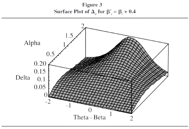 where $\texttt{Alpha}$ refers to $a_j$, $\texttt{Delta}$ refers to $\Delta_{ij}$, and $\texttt{Theta - Beta}$ refers to $\theta_i - b_j$. This allow researchers to quickly gauge the severity of the lack of invariance effects on the logit and probability scales and from a practical viewpoints, allows one to compute and visualize different lack of invariance effects on response probabilities and examinee true scores.
Lord’s $\mathcal{X}^2$ test (Lord, 1980): Note that $^*$ refers to the scale linked version. Formulation follows Battauz (2017)
\[H_0: v_{j, \texttt{old}} = v^*_{j, \texttt{new}} \equiv \begin{pmatrix} a_{j, \texttt{old}} \\ b_{j, \texttt{old}} \\ c_{j, \texttt{old}} \end{pmatrix} = \begin{pmatrix}a^*_{j, \texttt{new}} \\ b^*_{j, \texttt{new}} \\ c^*_{j, \texttt{new}}\end{pmatrix}\]\(\mathcal{X}_j^2 = \left(v_{k,\texttt{old}} - v^*_{j,\texttt{new}}\right)^T\left(\Sigma_{j, \texttt{old}}+\Sigma_{j, \texttt{new}}\right)^{-1}\left(v_{j,\texttt{old}}-v_{j, \texttt{new}}\right)\) where $\Sigma_{j, \texttt{old}}$ and $\Sigma_{j, \texttt{new}}$ represent the estimate covariance matrix for $v_{j, \texttt{old}}$ and $v_{j, \texttt{new}}$ respectively.
NLP Applications
Lalor et al (2016) questioned whether all items in a given test set are equal with regards to difficulty and discrimination power. They used Amazon Mechanical Turk works to annotate a sample of the Stanford Natural Language Inference Recognizing Textual Entailment. Researchers demonstrated IRT’s application to evaluating NLP systems. They trained an IRT model on human data to compare NLP system performance with the performance in a human population.
Lalor et al (2020) experimented on Natural Language Inference and Sentiment Analysis to show that the likelihood of answering a question correctly is impacted by the question difficulty. Logistic regression models used training set size and item difficulty as parameters to predict whether a deep neural network would label an item correctly. Neural model performance starts to look more human; as DNNs are trained with more data, “easy” examples are learned more quickly than hard examples.
Spurious Correlations
Models can achieve strong results by simply using the hypothesis of a premise-hypothesis pair and ignoring the premise entirely (Gururangan et al, 2018, Tsuchiya (2018), Poliak et al (2018))
Citations
Andersen (1970). Asymptotic Properties pf Conditional Maximum-Likelihood Estimators
Battauz (2017). On Wald Tests for Differential item Functioning Detection ↩
Bolt. (2002) A Monte Carlo Comparison of Parametric and Nonparametric Polytomous DIF Detection Methods
Breslau et al. (2008) Differential item functioning between ethnic groups in the epidemiological assessment of depression
Columbia University Mailman School of Public Health. (n.d.) Differential Item Functioning ↩
Columbia University Mailman School of Public Health. (n.d.). Item Response Theory.
Gururangan et al (2018). Annotation Artifacts in Natural Language Inference Data
Johnson (2007). Marginal Maximum Likelihood Estimation of Item Response Models in R.
Kang and Chen (2007). An Investigation of the Performance of the Generalized S-$X^2$ Item-Fit Index for Polytomous IRT Models
Kim and Cohen (2009). A Comparison of Lord’s Chi-Square, Raju’s Area Measures, and the Likelihood Ratio Test on Detection of Differential Item Functioning
Kim and Lee (2004). IRT Scale Linking Methods for Mixed-Format Tests
Lalor et al (2016). Building an Evaluation Scale using Item Response Theory
Lalor et al (2020). Understanding Deep Learning Performance through an Examination of Test Set Difficulty: A Psychometric Case Study
Lord (1980) Applications of item response theory to practical testing problems.
Poliak et al (2018). Hypothesis Only Baselines in Natural Language Inference
Robitzsch (2024). Bias-reduced Haebara and Stocking-Lord Linking in the Presence of Differential Item Functioning
Raju. (1988) The area between two item characteristic curves
Rupp and Zumbo. (2004) A note on how to quantify and report whether IRT parameter invariance holds: When Pearson correlations are not enough
Rupp and Zumbo. (2006) Understanding Parameter Invariance in Unidimensional IRT Models
Selçuk and Demir (2024) Comparison of item response theory ability and item parameters to classical and Bayesian estimation methods
Shepard, Camilli, and Williams, (1984). Accounting for Statistical Artifacts in Item Bias Research
Tsuchiya (2018). Performance Impact Caused by Hidden Bias of Training Data for Recognizing Textual Entailment
Weber et al. (2026) The stability of IRT parameters under several test equating conditions ↩
Wells (2021). Methods Based on Item Response Theory
Wu et al (2020). Variational Item Response Theory: Fast, Accurate, and Expressive
-
Asymptotic bias refers to the error between an expected statistical estimate and the true population value when the sample size grows infinitely large. ↩